8.3.22 arrayquantile

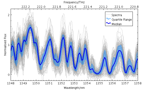
Displays a quantile or quantile range for a set of plotted X/Y array pairs. If a table contains one spectrum per row in array-valued wavelength and flux columns, this plotter can be used to display a median of all the spectra, or a range between two quantiles. Smoothing options are available to even out noise arising from the pixel binning.

For each row, the xs and ys arrays must be the same length as each other, but this plot type does not require all the arrays to be sampled into the same bins.

The algorithm calculates quantiles for all the X,Y points plotted in each column of pixels. This means that more densely sampled spectra have more influence on the output than sparser ones.

Note: in the current implementation, depending on the details of the configuration and the data, there may be some distortions or missing graphics near the edges of the plot. This may be improved in future releases, depending on feedback.

Usage Overview:

   layerN=arrayquantile colorN=<rrggbb>|red|blue|... transparencyN=0..1
                        quantilesN=<low-frac>[,<high-frac>] thickN=<pixels>
                        smoothN=+<width>|-<count>
                        kernelN=square|linear|epanechnikov|cos|cos2|gauss3|gauss6
                        joinN=none|polygon|lines horizontalN=true|false
                        xsN=<array-expr> ysN=<array-expr> inN=<table>
                        ifmtN=<in-format> istreamN=true|false icmdN=<cmds>

All the parameters listed here affect only the relevant layer, identified by the suffix N.

Example:

   stilts plot2plane in=xq100sub.fits xs=subWave ys=multiply(subFlux,1./mean(subFlux))
                     xlabel=Wavelength/nm ylabel='Normalised Flux'
                     x2func=SPEED_OF_LIGHT*1E9*1E-12/x x2label=Frequency/THz
                     layer1=lines shading1=density densemap1=greyscale
                     denseclip1=0.2,1 densefunc1=linear leglabel1=Spectra
                     layer_q13=ArrayQuantile color_q13=DodgerBlue transparency_q13=0.5
                     quantiles_q13=0.25,0.75 leglabel_q13='Quartile Range'
                     layer_med=ArrayQuantile color_med=blue join_med=lines leglabel_med=Median
                     legend=true legpos=0.95,0.95
                     xpix=600 ypix=380
                     xmin=1348 xmax=1358 ymin=-0.2 ymax=2.2

colorN = <rrggbb>|red|blue|...       (Color)

The color of plotted data, given by name or as a hexadecimal RGB value.

The standard plotting colour names are red, blue, green, grey, magenta, cyan, orange, pink, yellow, black, light_grey, white. However, many other common colour names (too many to list here) are also understood. The list currently contains those colour names understood by most web browsers, from AliceBlue to YellowGreen, listed e.g. in the Extended color keywords section of the CSS3 standard.

Alternatively, a six-digit hexadecimal number RRGGBB may be supplied, optionally prefixed by "#" or "0x", giving red, green and blue intensities, e.g. "ff00ff", "#ff00ff" or "0xff00ff" for magenta.

[Default: red]

horizontalN = true|false       (Boolean)

Determines whether the trace bins are horizontal or vertical. If true, y quantiles are calculated for each pixel column, and if false, x quantiles are calculated for each pixel row.

[Default: true]

icmdN = <cmds>       (ProcessingStep[])

Specifies processing to be performed on the layer N input table as specified by parameter inN. The value of this parameter is one or more of the filter commands described in Section 6.1. If more than one is given, they must be separated by semicolon characters (";"). This parameter can be repeated multiple times on the same command line to build up a list of processing steps. The sequence of commands given in this way defines the processing pipeline which is performed on the table.

Commands may alternatively be supplied in an external file, by using the indirection character '@'. Thus a value of "@filename" causes the file filename to be read for a list of filter commands to execute. The commands in the file may be separated by newline characters and/or semicolons, and lines which are blank or which start with a '#' character are ignored. A backslash character '\' at the end of a line joins it with the following line.

ifmtN = <in-format>       (String)

Specifies the format of the input table as specified by parameter inN. The known formats are listed in Section 5.1.1. This flag can be used if you know what format your table is in. If it has the special value (auto) (the default), then an attempt will be made to detect the format of the table automatically. This cannot always be done correctly however, in which case the program will exit with an error explaining which formats were attempted. This parameter is ignored for scheme-specified tables.

[Default: (auto)]

inN = <table>       (StarTable)

The location of the input table. This may take one of the following forms:

• A filename.
• A URL.
• The special value "-", meaning standard input. In this case the input format must be given explicitly using the ifmtN parameter. Note that not all formats can be streamed in this way.
• A scheme specification of the form :<scheme-name>:<scheme-args>.
• A system command line with either a "<" character at the start, or a "|" character at the end ("<syscmd" or "syscmd|"). This executes the given pipeline and reads from its standard output. This will probably only work on unix-like systems.

In any case, compressed data in one of the supported compression formats (gzip, Unix compress or bzip2) will be decompressed transparently.

istreamN = true|false       (Boolean)

If set true, the input table specified by the inN parameter will be read as a stream. It is necessary to give the ifmtN parameter in this case. Depending on the required operations and processing mode, this may cause the read to fail (sometimes it is necessary to read the table more than once). It is not normally necessary to set this flag; in most cases the data will be streamed automatically if that is the best thing to do. However it can sometimes result in less resource usage when processing large files in certain formats (such as VOTable). This parameter is ignored for scheme-specified tables.

[Default: false]

joinN = none|polygon|lines       (QJoin)

Defines the graphical style for connecting distinct quantile values. If smoothed samples are packed more closely than the pixel grid the option chosen here doesn't make much difference, but if there are gaps in the data along the sampled axis, it's useful to have a guide to the eye to join one quantile determination to the next.

The available options are:

• none: displayed quantile ranges are not joined
• polygon: the area between a line connecting the upper quantiles and a line connecting the lower quantiles is filled
• lines: a line of thickness given by thick is drawn from the center of each quantile range to the next

[Default: polygon]

kernelN = square|linear|epanechnikov|cos|cos2|gauss3|gauss6       (Kernel1dShape)

The functional form of the smoothing kernel. The functions listed refer to the unscaled shape; all kernels are normalised to give a total area of unity.

The available options are:

• square: Uniform value: f(x)=1, |x|=0..1
• linear: Triangle: f(x)=1-|x|, |x|=0..1
• epanechnikov: Parabola: f(x)=1-x*x, |x|=0..1
• cos: Cosine: f(x)=cos(x*pi/2), |x|=0..1
• cos2: Cosine squared: f(x)=cos^2(x*pi/2), |x|=0..1
• gauss3: Gaussian truncated at 3.0 sigma: f(x)=exp(-x*x/2), |x|=0..3
• gauss6: Gaussian truncated at 6.0 sigma: f(x)=exp(-x*x/2), |x|=0..6

[Default: epanechnikov]

quantilesN = <low-frac>[,<high-frac>]       (Subrange)

Defines the quantile or quantile range of values that should be marked in each pixel column (or row). The value may be a single number in the range 0..1 indicating the quantile which should be marked. Alternatively, it may be a pair of numbers, each in the range 0..1, separated by commas (<lo>,<hi>) indicating two quantile lines bounding an area to be filled. A pair of equal values "a,a" is equivalent to the single value "a". The default is 0.5, which means to mark the median value in each column, and could equivalently be specified 0.5,0.5.

[Default: 0.5]

smoothN = +<width>|-<count>       (BinSizer)

Configures the smoothing width. This is the characteristic width of the kernel function to be convolved with the density in one dimension to smooth the quantile function.

If the supplied value is a positive number it is interpreted as a fixed width in the data coordinates of the X axis (if the X axis is logarithmic, the value is a fixed factor). If it is a negative number, then it will be interpreted as the approximate number of smooothing widths that fit in the width of the visible plot (i.e. plot width / smoothing width). If the value is zero, no smoothing is applied.

When setting this value graphically, you can use either the slider to adjust the bin count or the numeric entry field to fix the bin width.

[Default: 0]

thickN = <pixels>       (Integer)

Sets the minimum extent of the markers that are plotted in each pixel column (or row) to indicate the designated value range. If the range is zero sized (quantiles specifies a single value rather than a pair) this will give the actual thickness of the plotted line. If the range is non-zero however, the line may be thicker than this in places according to the quantile positions.

[Default: 3]

transparencyN = 0..1       (Double)

Transparency with which components are plotted, in the range 0 (opaque) to 1 (invisible). The value is 1-alpha.

[Default: 0]

xsN = <array-expr>       (String)

Array giving the X coordinate array for each line. In most cases, if a blank value is supplied but Y values are present then a suitable linear sequence, of the same length as the Y array, is assumed.

The value is an array-valued algebraic expression based on column names as described in Section 10. Some of the functions in the Arrays class may be useful here.

ysN = <array-expr>       (String)

Array giving the Y coordinate array for each line. In most cases, if a blank value is supplied but X values are present then a suitable linear sequence, of the same length as the X array, is assumed.

The value is an array-valued algebraic expression based on column names as described in Section 10. Some of the functions in the Arrays class may be useful here.