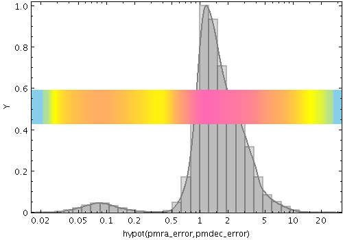
8.3.34 densogram

Represents smoothed density of data values along the horizontal axis using a colourmap. This is like a Kernel Density Estimate (smoothed histogram with bins 1 pixel wide), but instead of representing the data extent vertically as bars or a line, values are represented by a fixed-size pixel-width column of a colour from a colour map. A smoothing kernel, whose width and shape may be varied, is applied to each data point.

A weighting may be applied to the calculated levels by supplying the weight coordinate. In this case you can choose how these weights are aggregated in each pixel bin using the combine parameter. The result is something like a smoothed version of the corresponding weighted histogram. Note that some combinations of the available parameters (e.g. a normalised cumulative median-aggregated KDE) may not make much visual sense.

This is a rather unconventional way to represent density data, and this plotting mode is probably not very useful. But hey, nobody's forcing you to use it.

Usage Overview:

   layerN=densogram colorN=<rrggbb>|red|blue|... smoothN=+<width>|-<count>
                    sidewaysN=true|false
                    kernelN=square|linear|epanechnikov|cos|cos2|gauss3|gauss6
                    densemapN=<map-name>|<color>-<color>[-<color>...]
                    denseclipN=<lo>,<hi> denseflipN=true|false
                    densequantN=<number> densesubN=<lo>,<hi>
                    densefuncN=log|linear|histogram|histolog|sqrt|square|acos|cos
                    cumulativeN=none|forward|reverse sizeN=<pixels>
                    posN=<fraction> xN=<num-expr> weightN=<num-expr>
                    inN=<table> ifmtN=<in-format> istreamN=true|false
                    icmdN=<cmds>

All the parameters listed here affect only the relevant layer, identified by the suffix N.

Example:

   stilts plot2plane in=tgas_source.fits x=hypot(pmra_error,pmdec_error)
                     xlog=true normalise=maximum
                     color=grey layer1=histogram layer2=kde
                     layer3=densogram densemap3=skyblue-yellow-hotpink densefunc3=log
                     size3=50 pos3=0.5

colorN = <rrggbb>|red|blue|...       (Color)

The color of plotted data, given by name or as a hexadecimal RGB value.

The standard plotting colour names are red, blue, green, grey, magenta, cyan, orange, pink, yellow, black, light_grey, white. However, many other common colour names (too many to list here) are also understood. The list currently contains those colour names understood by most web browsers, from AliceBlue to YellowGreen, listed e.g. in the Extended color keywords section of the CSS3 standard.

Alternatively, a six-digit hexadecimal number RRGGBB may be supplied, optionally prefixed by "#" or "0x", giving red, green and blue intensities, e.g. "ff00ff", "#ff00ff" or "0xff00ff" for magenta.

[Default: red]

cumulativeN = none|forward|reverse       (Cumulation)

If set to forward/reverse the histogram bars plotted are calculated cumulatively; each bin includes the counts from all previous bins working up/down the independent axis.

Note that setting cumulative plotting may not make much sense with some other parameter values, for instance averaging aggregation modes.

For reasons of backward compatibility, the values true and false may be used as aliases for forward and none.

The available options are:

• none: The value plotted for each bin uses the samples accumulated in that bin.
• forward: The value plotted for each bin uses the samples accumulated all the way from negative infinity to that bin.
• reverse: The value plotted for each bin uses the samples accumulated all the way from positive infinity to that bin.

[Default: none]

denseclipN = <lo>,<hi>       (Subrange)

Defines a subrange of the colour ramp to be used for Density shading. The value is specified as a (low,high) comma-separated pair of two numbers between 0 and 1.

If the full range 0,1 is used, the whole range of colours specified by the selected shader will be used. But if for instance a value of 0,0.5 is given, only those colours at the left hand end of the ramp will be seen.

If the null (default) value is chosen, a default clip will be used. This generally covers most or all of the range 0-1 but for colour maps which fade to white, a small proportion of the lower end may be excluded, to ensure that all the colours are visually distinguishable from a white background. This default is usually a good idea if the colour map is being used with something like a scatter plot, where markers are plotted against a white background. However, for something like a density map when the whole plotting area is tiled with colours from the map, it may be better to supply the whole range 0,1 explicitly.

denseflipN = true|false       (Boolean)

If true, the colour map on the Density axis will be reversed.

[Default: false]

densefuncN = log|linear|histogram|histolog|sqrt|square|acos|cos       (Scaling)

Defines the way that values in the Density range are mapped to the selected colour ramp.

The available options are:

• log: Logarithmic scaling
• linear: Linear scaling
• histogram: Scaling follows data distribution, with linear axis
• histolog: Scaling follows data distribution, with logarithmic axis
• sqrt: Square root scaling
• square: Square scaling
• acos: Arccos Scaling
• cos: Cos Scaling

For all these options, the full range of data values is used, and displayed on the colour bar if applicable (though it can be restricted using the densesub option) The Linear, Log, Square and Sqrt options just apply the named function to the full data range. The histogram options on the other hand use a scaling function that corresponds to the actual distribution of the data, so that there are about the same number of points (or pixels, or whatever is being scaled) of each colour. The histogram options are somewhat more expensive, but can be a good choice if you are exploring data whose distribution is unknown or not well-behaved over its min-max range. The Histogram and HistoLog options both assign the colours in the same way, but they display the colour ramp with linear or logarithmic annotation respectively; the HistoLog option also ignores non-positive values.

[Default: linear]

densemapN = <map-name>|<color>-<color>[-<color>...]       (Shader)

Color map used for Density axis shading.

A mixed bag of colour ramps are available as listed in Section 8.7: inferno, magma, plasma, viridis, cividis, cubehelix, sron, rainbow, rainbow2, rainbow3, pastel, cosmic, ember, gothic, rainforest, voltage, bubblegum, gem, chroma, sunset, neon, tropical, accent, gnuplot, gnuplot2, specxby, set1, paired, hotcold, guppy, iceburn, redshift, pride, rdbu, piyg, brbg, cyan-magenta, red-blue, brg, heat, cold, light, greyscale, colour, standard, bugn, bupu, orrd, pubu, purd, painbow, huecl, infinity, hue, intensity, rgb_red, rgb_green, rgb_blue, hsv_h, hsv_s, hsv_v, yuv_y, yuv_u, yuv_v, scale_hsv_s, scale_hsv_v, scale_yuv_y, mask, blacker, whiter, transparency. Note: many of these, including rainbow-like ones, are frowned upon by the visualisation community.

You can also construct your own custom colour map by giving a sequence of colour names separated by minus sign ("-") characters. In this case the ramp is a linear interpolation between each pair of colours named, using the same syntax as when specifying a colour value. So for instance "yellow-hotpink-#0000ff" would shade from yellow via hot pink to blue.

[Default: inferno]

densequantN = <number>       (Double)

Allows the colour map used for the Density axis to be quantised. If an integer value N is chosen then the colour map will be viewed as N discrete evenly-spaced levels, so that only N different colours will appear in the plot. This can be used to generate a contour-like effect, and may make it easier to trace the boundaries of regions of interest by eye.

If left blank, the colour map is nominally continuous (though in practice it may be quantised to a medium-sized number like 256).

densesubN = <lo>,<hi>       (Subrange)

Defines a normalised adjustment to the data range of the Density axis. The value may be specified as a comma-separated pair of two numbers, giving the lower and upper bounds of the range of of interest respectively. This sub-range is applied to the data range that would otherwise be used, either automatically calculated or explicitly supplied; zero corresponds to the lower bound and one to the upper.

The default value "0,1" therefore has no effect. The range could be restricted to its lower half with the value 0,0.5.

[Default: 0,1]

icmdN = <cmds>       (ProcessingStep[])

Specifies processing to be performed on the layer N input table as specified by parameter inN. The value of this parameter is one or more of the filter commands described in Section 6.1. If more than one is given, they must be separated by semicolon characters (";"). This parameter can be repeated multiple times on the same command line to build up a list of processing steps. The sequence of commands given in this way defines the processing pipeline which is performed on the table.

Commands may alternatively be supplied in an external file, by using the indirection character '@'. Thus a value of "@filename" causes the file filename to be read for a list of filter commands to execute. The commands in the file may be separated by newline characters and/or semicolons, and lines which are blank or which start with a '#' character are ignored. A backslash character '\' at the end of a line joins it with the following line.

ifmtN = <in-format>       (String)

Specifies the format of the input table as specified by parameter inN. The known formats are listed in Section 5.1.1. This flag can be used if you know what format your table is in. If it has the special value (auto) (the default), then an attempt will be made to detect the format of the table automatically. This cannot always be done correctly however, in which case the program will exit with an error explaining which formats were attempted. This parameter is ignored for scheme-specified tables.

[Default: (auto)]

inN = <table>       (StarTable)

The location of the input table. This may take one of the following forms:

• A filename.
• A URL.
• The special value "-", meaning standard input. In this case the input format must be given explicitly using the ifmtN parameter. Note that not all formats can be streamed in this way.
• A scheme specification of the form :<scheme-name>:<scheme-args>.
• A system command line with either a "<" character at the start, or a "|" character at the end ("<syscmd" or "syscmd|"). This executes the given pipeline and reads from its standard output. This will probably only work on unix-like systems.

In any case, compressed data in one of the supported compression formats (gzip, Unix compress or bzip2) will be decompressed transparently.

istreamN = true|false       (Boolean)

If set true, the input table specified by the inN parameter will be read as a stream. It is necessary to give the ifmtN parameter in this case. Depending on the required operations and processing mode, this may cause the read to fail (sometimes it is necessary to read the table more than once). It is not normally necessary to set this flag; in most cases the data will be streamed automatically if that is the best thing to do. However it can sometimes result in less resource usage when processing large files in certain formats (such as VOTable). This parameter is ignored for scheme-specified tables.

[Default: false]

kernelN = square|linear|epanechnikov|cos|cos2|gauss3|gauss6       (Kernel1dShape)

The functional form of the smoothing kernel. The functions listed refer to the unscaled shape; all kernels are normalised to give a total area of unity.

The available options are:

• square: Uniform value: f(x)=1, |x|=0..1
• linear: Triangle: f(x)=1-|x|, |x|=0..1
• epanechnikov: Parabola: f(x)=1-x*x, |x|=0..1
• cos: Cosine: f(x)=cos(x*pi/2), |x|=0..1
• cos2: Cosine squared: f(x)=cos^2(x*pi/2), |x|=0..1
• gauss3: Gaussian truncated at 3.0 sigma: f(x)=exp(-x*x/2), |x|=0..3
• gauss6: Gaussian truncated at 6.0 sigma: f(x)=exp(-x*x/2), |x|=0..6

[Default: epanechnikov]

posN = <fraction>       (Double)

Determines where on the plot region the density bar appears. The value should be in the range 0..1; zero corresponds to the bottom of the plot and one to the top.

[Default: 0.05]

sidewaysN = true|false       (Boolean)

When set to the default value of false, the quantity being accumulated is on the the horizontal axis and the frequency is represented vertically as usual. If set true the quantity accumulated is on the vertical axis, and the frequency is represented horizontally, so that the chart is displayed reflected in the X=Y line.

[Default: false]

sizeN = <pixels>       (Integer)

Height of the density bar in pixels.

[Default: 12]

smoothN = +<width>|-<count>       (BinSizer)

Configures the smoothing width for kernel density estimation. This is the characteristic width of the kernel function to be convolved with the density to produce the visible plot.

If the supplied value is a positive number it is interpreted as a fixed width in the data coordinates of the X axis (if the X axis is logarithmic, the value is a fixed factor). If it is a negative number, then it will be interpreted as the approximate number of smooothing widths that fit in the width of the visible plot (i.e. plot width / smoothing width). If the value is zero, no smoothing is applied.

When setting this value graphically, you can use either the slider to adjust the bin count or the numeric entry field to fix the bin width.

[Default: -100]

weightN = <num-expr>       (String)

Weighting of data points. If supplied, each point contributes a value to the histogram equal to the data value multiplied by this coordinate. If not supplied, the effect is the same as supplying a fixed value of one.

The value is a numeric algebraic expression based on column names as described in Section 10.

xN = <num-expr>       (String)

Horizontal coordinate.

The value is a numeric algebraic expression based on column names as described in Section 10.