A.4.5.22 KDE Form

The KDE form () plots a discrete Kernel Density Estimate giving a smoothed frequency of data values along the horizontal axis, using a fixed-width smoothing kernel. (for a variable-bandwidth kernel, see KNN). This is a generalisation of a histogram in which the bins are always 1 pixel wide, and a smoothing kernel is applied to each bin. The width and shape of the kernel may be varied.

This is suitable for cases where the division into discrete bins done by a normal histogram is unnecessary or troublesome.

Note this is not a true Kernel Density Estimate, since, for performance reasons, the smoothing is applied to the (pixel-width) bins rather than to each data sample. The deviation from a true KDE caused by this quantisation will be at the pixel level, hence in most cases not visually apparent.

This form may be used in the Histogram, Plane or Time plot windows.

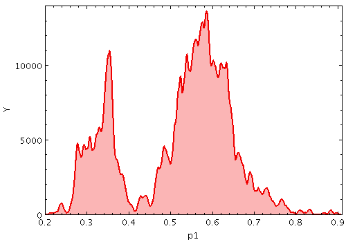
Example KDE plot

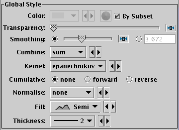
KDE form configuration panel

These options always appear in the form configuration panel:

Colour

Selects the basic colour for the dataset.

Transparency

Adjusts the transparency of the bars or line. For bar styles which are already partially transparent, this fades them further.

Combine

Defines how values contributing to the same bin are combined together to produce the value assigned to that bin, and hence its height. The bins in this case are 1-pixel wide, so lack much physical significance. This means that while some combination modes, such as sum-per-unit and mean make sense, others such as sum do not.

The combined values are those given by the Weight coordinate, but if no weight is supplied, a weighting of unity is assumed.

The available options are:

• sum: the sum of all the combined values per bin
• sum-per-unit: the sum of all the combined values per unit of bin size
• count: the number of non-blank values per bin (weight is ignored)
• count-per-unit: the number of non-blank values per unit of bin size (weight is ignored)
• mean: the mean of the combined values
• median: the median of the combined values (may be slow)
• q1: the first quartile of the combined values (may be slow)
• q3: the third quartile of the combined values (may be slow)
• min: the minimum of all the combined values
• max: the maximum of all the combined values
• stdev: the sample standard deviation of the combined values
• hit: 1 if any values present, NaN otherwise (weight is ignored)

Fill

Determines how the density function is represented. The options are:

• solid: area between level and axis is filled with solid colour
• line: level is marked by a wiggly line
• semi: level is marked by a wiggly line, and area below it is filled with a transparent colour

Thickness

Controls line thickness where applicable. This is only relevant for bar styles that draw a finite thickness line, so has no effect for solid filling.

Smoothing

Configures the smoothing width for kernel density estimation. This is the characteristic width of the kernel function to be convolved with the density to produce the visible plot.

Sliding the slider to the right makes the kernel width larger. The width in data units is shown in the text field on the right (if the X axis is logarithmic, this is a factor). Alternatively you can click the radio button near the text field, and enter the width in data units directly.

Kernel

The functional form of the smoothing kernel. The functions listed refer to the unscaled shape; all kernels are normalised to give a total area of unity.

The available options are:

• square: Uniform value: f(x)=1, |x|=0..1
• linear: Triangle: f(x)=1-|x|, |x|=0..1
• epanechnikov: Parabola: f(x)=1-x*x, |x|=0..1
• cos: Cosine: f(x)=cos(x*pi/2), |x|=0..1
• cos2: Cosine squared: f(x)=cos^2(x*pi/2), |x|=0..1
• gauss3: Gaussian truncated at 3.0 sigma: f(x)=exp(-x*x/2), |x|=0..3
• gauss6: Gaussian truncated at 6.0 sigma: f(x)=exp(-x*x/2), |x|=0..6

Cumulative

If set to forward or reverse, the heights are plotted cumulatively; each bin includes the counts from all previous bins in the direction of negative or positive infinity.

Normalise

Defines how, if at all, the bars are normalised. The available options are:

• none: No normalisation is performed.
• area: The total area of histogram bars is normalised to unity. For cumulative plots, this behaves like height.
• unit: Histogram bars are scaled by the inverse of the bin width in data units. For cumulative plots, this behaves like none.
• maximum: The height of the tallest histogram bar is normalised to unity. For cumulative plots, this behaves like height.
• height: The total height of histogram bars is normalised to unity.

When used in the Time plot only, additional options per_second, per_day etc are available corresponding to the frequency over the named time unit.