8.3.28 grid

Plots 2-d data aggregated into rectangular cells. You can optionally use a weighting for the points, and you can configure how the values are combined to produce the output pixel values (colours). You can use this plotter in various ways, including as a 2-d histogram or weighted density map, or to plot gridded data.

The X and Y dimensions of the grid cells (or equivalently histogram bins) can be configured either in terms of the data coordinates or relative to the plot dimensions.

The way that data values are mapped to colours is usually controlled by options at the level of the plot itself, rather than by per-layer configuration.

Usage Overview:

   layerN=grid xbinsizeN=+<extent>|-<count> ybinsizeN=+<extent>|-<count>
               combineN=sum|sum-per-unit|count|... transparencyN=0..1
               xphaseN=<number> yphaseN=<number> <pos-coord-paramsN>
               weightN=<num-expr> inN=<table> ifmtN=<in-format>
               istreamN=true|false icmdN=<cmds>

All the parameters listed here affect only the relevant layer, identified by the suffix N.

Positional Coordinate Parameters:

The positional coordinates <pos-coord-paramsN> give a position for each row of the input table. Their form depends on the plot geometry, i.e. which plotting command is used. For a plane plot (plot2plane) the parameters would be xN and yN. The coordinate parameter values are in all cases strings interpreted as numeric expressions based on column names. These can be column names, fixed values or algebraic expressions as described in Section 10.

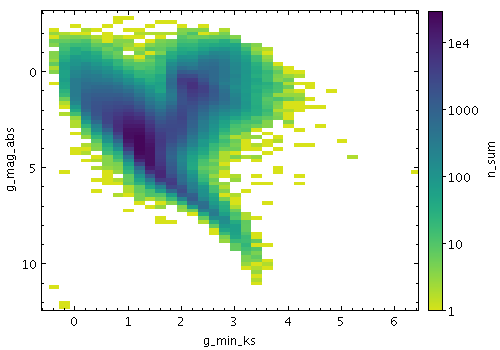
Example:

   stilts plot2plane layer1=grid in1=gk_hess.fits x1=g_min_ks y1=g_mag_abs
                     weight1=n combine1=sum xbinsize1=0.2 ybinsize1=0.2 xphase1=0.5 yphase1=0.5
                     yflip=true auxfunc=log auxmap=viridis

combineN = sum|sum-per-unit|count|...       (Combiner)

Defines how values contributing to the same grid cell are combined together to produce the value assigned to that cell, and hence its colour. The combined values are the weights, but if the weight coordinate is left blank, a weighting of unity is assumed.

The available options are:

• sum: the sum of all the combined values per bin
• sum-per-unit: the sum of all the combined values per unit of bin size
• count: the number of non-blank values per bin (weight is ignored)
• count-per-unit: the number of non-blank values per unit of bin size (weight is ignored)
• mean: the mean of the combined values
• median: the median
• q1: first quartile
• q3: third quartile
• min: the minimum of all the combined values
• max: the maximum of all the combined values
• stdev: the sample standard deviation of the combined values
• stdev_pop: the population standard deviation of the combined values
• hit: 1 if any values present, NaN otherwise (weight is ignored)

[Default: mean]

icmdN = <cmds>       (ProcessingStep[])

Specifies processing to be performed on the layer N input table as specified by parameter inN. The value of this parameter is one or more of the filter commands described in Section 6.1. If more than one is given, they must be separated by semicolon characters (";"). This parameter can be repeated multiple times on the same command line to build up a list of processing steps. The sequence of commands given in this way defines the processing pipeline which is performed on the table.

Commands may alternatively be supplied in an external file, by using the indirection character '@'. Thus a value of "@filename" causes the file filename to be read for a list of filter commands to execute. The commands in the file may be separated by newline characters and/or semicolons, and lines which are blank or which start with a '#' character are ignored. A backslash character '\' at the end of a line joins it with the following line.

ifmtN = <in-format>       (String)

Specifies the format of the input table as specified by parameter inN. The known formats are listed in Section 5.1.1. This flag can be used if you know what format your table is in. If it has the special value (auto) (the default), then an attempt will be made to detect the format of the table automatically. This cannot always be done correctly however, in which case the program will exit with an error explaining which formats were attempted. This parameter is ignored for scheme-specified tables.

[Default: (auto)]

inN = <table>       (StarTable)

The location of the input table. This may take one of the following forms:

• A filename.
• A URL.
• The special value "-", meaning standard input. In this case the input format must be given explicitly using the ifmtN parameter. Note that not all formats can be streamed in this way.
• A scheme specification of the form :<scheme-name>:<scheme-args>.
• A system command line with either a "<" character at the start, or a "|" character at the end ("<syscmd" or "syscmd|"). This executes the given pipeline and reads from its standard output. This will probably only work on unix-like systems.

In any case, compressed data in one of the supported compression formats (gzip, Unix compress or bzip2) will be decompressed transparently.

istreamN = true|false       (Boolean)

If set true, the input table specified by the inN parameter will be read as a stream. It is necessary to give the ifmtN parameter in this case. Depending on the required operations and processing mode, this may cause the read to fail (sometimes it is necessary to read the table more than once). It is not normally necessary to set this flag; in most cases the data will be streamed automatically if that is the best thing to do. However it can sometimes result in less resource usage when processing large files in certain formats (such as VOTable). This parameter is ignored for scheme-specified tables.

[Default: false]

transparencyN = 0..1       (Double)

Transparency with which components are plotted, in the range 0 (opaque) to 1 (invisible). The value is 1-alpha.

[Default: 0]

weightN = <num-expr>       (String)

Weighting of data points. If supplied, each point contributes a value to the histogram equal to the data value multiplied by this coordinate. If not supplied, the effect is the same as supplying a fixed value of one.

The value is a numeric algebraic expression based on column names as described in Section 10.

xbinsizeN = +<extent>|-<count>       (BinSizer)

Configures the extent of the density grid bins on the X axis.

If the supplied value is a positive number it is interpreted as a fixed size in data coordinates (if the X axis is logarithmic, the value is a fixed factor). If it is a negative number, then it will be interpreted as the approximate number of bins to display across the plot in the X direction (though an attempt is made to use only round numbers for bin sizes).

When setting this value graphically, you can use either the slider to adjust the bin count or the numeric entry field to fix the bin size.

[Default: -30]

xphaseN = <number>       (Double)

Controls where the zero point on the X axis is set. For instance if your bin size is 1, this value controls whether bin boundaries are at 0, 1, 2, .. or 0.5, 1.5, 2.5, ... etc.

A value of 0 (or any integer) will result in a bin boundary at X=0 (linear X axis) or X=1 (logarithmic X axis). A fractional value will give a bin boundary at that value multiplied by the bin width.

[Default: 0]

ybinsizeN = +<extent>|-<count>       (BinSizer)

Configures the extent of the density grid bins on the Y axis.

If the supplied value is a positive number it is interpreted as a fixed size in data coordinates (if the Y axis is logarithmic, the value is a fixed factor). If it is a negative number, then it will be interpreted as the approximate number of bins to display across the plot in the Y direction (though an attempt is made to use only round numbers for bin sizes).

When setting this value graphically, you can use either the slider to adjust the bin count or the numeric entry field to fix the bin size.

[Default: -30]

yphaseN = <number>       (Double)

Controls where the zero point on the Y axis is set. For instance if your bin size is 1, this value controls whether bin boundaries are at 0, 1, 2, .. or 0.5, 1.5, 2.5, ... etc.

A value of 0 (or any integer) will result in a bin boundary at X=0 (linear X axis) or X=1 (logarithmic X axis). A fractional value will give a bin boundary at that value multiplied by the bin width.

[Default: 0]