8.3.27 contour

Plots position density contours. This provides another way (alongside the auto, density and weighted shading modes) to visualise the characteristics of overdense regions in a crowded plot. It's not very useful if you just have a few points.

A weighting may optionally be applied to the quantity being contoured. To do this, provide a non-blank value for the weight coordinate, and use the combine parameter to define how the weights are combined (sum, mean, etc).

The contours are currently drawn as pixels rather than lines so they don't look very beautiful in exported vector output formats (PDF, PostScript). This may be improved in the future.

Usage Overview:

   layerN=contour colorN=<rrggbb>|red|blue|...
                  combineN=sum|mean|median|stdev|min|max|count
                  nlevelN=<int-value> smoothN=<pixels> thickN=<pixels>
                  scalingN=linear|log|equal zeroN=<number> <pos-coord-paramsN>
                  weightN=<num-expr> inN=<table> ifmtN=<in-format>
                  istreamN=true|false icmdN=<cmds>

All the parameters listed here affect only the relevant layer, identified by the suffix N.

Positional Coordinate Parameters:

The positional coordinates <pos-coord-paramsN> give a position for each row of the input table. Their form depends on the plot geometry, i.e. which plotting command is used. For a plane plot (plot2plane) the parameters would be xN and yN. The coordinate parameter values are in all cases strings interpreted as numeric expressions based on column names. These can be column names, fixed values or algebraic expressions as described in Section 10.

Example:

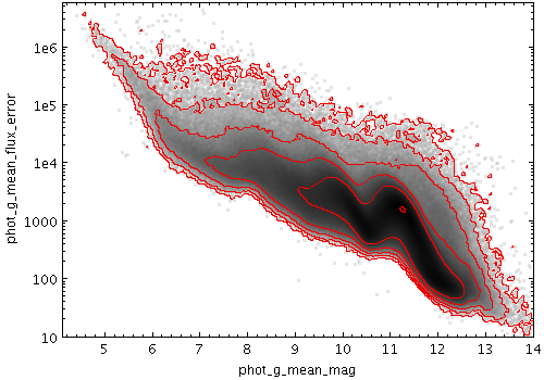
   stilts plot2plane in=tgas_source.fits x=phot_g_mean_mag y=phot_g_mean_flux_error
                     ylog=true xmax=14 ymin=10
                     layer1=mark shading1=density densemap1=greyscale
                     layer2=contour scaling2=log nlevel=6

colorN = <rrggbb>|red|blue|...       (Color)

The color of plotted data, given by name or as a hexadecimal RGB value.

The standard plotting colour names are red, blue, green, grey, magenta, cyan, orange, pink, yellow, black, light_grey, white. However, many other common colour names (too many to list here) are also understood. The list currently contains those colour names understood by most web browsers, from AliceBlue to YellowGreen, listed e.g. in the Extended color keywords section of the CSS3 standard.

Alternatively, a six-digit hexadecimal number RRGGBB may be supplied, optionally prefixed by "#" or "0x", giving red, green and blue intensities, e.g. "ff00ff", "#ff00ff" or "0xff00ff" for magenta.

[Default: red]

combineN = sum|mean|median|stdev|min|max|count       (Combiner)

Defines the way that the weight values are combined when generating the value grid for which the contours will be plotted. If a weighting is supplied, the most useful values are mean which traces the mean values of a quantity and sum which traces the weighted sum. Other values such as median are of dubious validity because of the way that the smoothing is done.

This value is ignored if the weighting coordinate weight is not set.

The available options are:

• sum: the sum of all the combined values per bin
• mean: the mean of the combined values
• median: the median
• stdev: the sample standard deviation of the combined values
• min: the minimum of all the combined values
• max: the maximum of all the combined values
• count: the number of non-blank values per bin (weight is ignored)

[Default: sum]

icmdN = <cmds>       (ProcessingStep[])

Specifies processing to be performed on the layer N input table as specified by parameter inN. The value of this parameter is one or more of the filter commands described in Section 6.1. If more than one is given, they must be separated by semicolon characters (";"). This parameter can be repeated multiple times on the same command line to build up a list of processing steps. The sequence of commands given in this way defines the processing pipeline which is performed on the table.

Commands may alternatively be supplied in an external file, by using the indirection character '@'. Thus a value of "@filename" causes the file filename to be read for a list of filter commands to execute. The commands in the file may be separated by newline characters and/or semicolons, and lines which are blank or which start with a '#' character are ignored. A backslash character '\' at the end of a line joins it with the following line.

ifmtN = <in-format>       (String)

Specifies the format of the input table as specified by parameter inN. The known formats are listed in Section 5.1.1. This flag can be used if you know what format your table is in. If it has the special value (auto) (the default), then an attempt will be made to detect the format of the table automatically. This cannot always be done correctly however, in which case the program will exit with an error explaining which formats were attempted. This parameter is ignored for scheme-specified tables.

[Default: (auto)]

inN = <table>       (StarTable)

The location of the input table. This may take one of the following forms:

• A filename.
• A URL.
• The special value "-", meaning standard input. In this case the input format must be given explicitly using the ifmtN parameter. Note that not all formats can be streamed in this way.
• A scheme specification of the form :<scheme-name>:<scheme-args>.
• A system command line with either a "<" character at the start, or a "|" character at the end ("<syscmd" or "syscmd|"). This executes the given pipeline and reads from its standard output. This will probably only work on unix-like systems.

In any case, compressed data in one of the supported compression formats (gzip, Unix compress or bzip2) will be decompressed transparently.

istreamN = true|false       (Boolean)

If set true, the input table specified by the inN parameter will be read as a stream. It is necessary to give the ifmtN parameter in this case. Depending on the required operations and processing mode, this may cause the read to fail (sometimes it is necessary to read the table more than once). It is not normally necessary to set this flag; in most cases the data will be streamed automatically if that is the best thing to do. However it can sometimes result in less resource usage when processing large files in certain formats (such as VOTable). This parameter is ignored for scheme-specified tables.

[Default: false]

nlevelN = <int-value>       (Integer)

Number of countour lines drawn. In fact, this is an upper limit; if there is not enough variation in the plot's density, then fewer contour lines will be drawn.

[Default: 5]

scalingN = linear|log|equal       (LevelMode)

How the smoothed density is treated before contour levels are determined.

The available options are:

• linear: levels are equally spaced
• log: level logarithms are equally spaced
• equal: levels are spaced to provide equal-area inter-contour regions

[Default: linear]

smoothN = <pixels>       (Integer)

The linear size of the smoothing kernel applied to the density before performing the contour determination. If set too low the contours will be too crinkly, and if too high they will lose definition. Smoothing currently uses an approximately Gaussian kernel for extensive combination modes (count, sum) or a circular top hat for intensive modes (weighted mean).

[Default: 5]

thickN = <pixels>       (Integer)

Thickness of plotted line in pixels.

[Default: 1]

weightN = <num-expr>       (String)

Weighting of data points. If supplied, each point contributes a value to the histogram equal to the data value multiplied by this coordinate. If not supplied, the effect is the same as supplying a fixed value of one.

The value is a numeric algebraic expression based on column names as described in Section 10.

zeroN = <number>       (Double)

Determines the level at which the first contour (and hence all the others, which are separated from it by a fixed amount) are drawn.

[Default: 1]