3 Vectors in 2D and 3D
So far we’ve been looking at motion in one dimension. However, in general we are interested in motion in two and three dimensions. To describe motion in two and three dimensions it is very convenient to use vectors.
Vectors will be used extensively throughout your physics degree. Later on you will find that vectors can be generalised in all sorts of interesting ways so it is important to have a solid understanding of the fundamentals, even if they can seem deceptively straightforward at first. You’ll find that surprisingly deep insights can often come from seemingly simple ideas!
In mechanics we will use vectors to describe things like the position of an object, its speed and direction of motion (velocity), and acceleration.
3.1 Vector properties and algebra
3.1.1 Vector addition
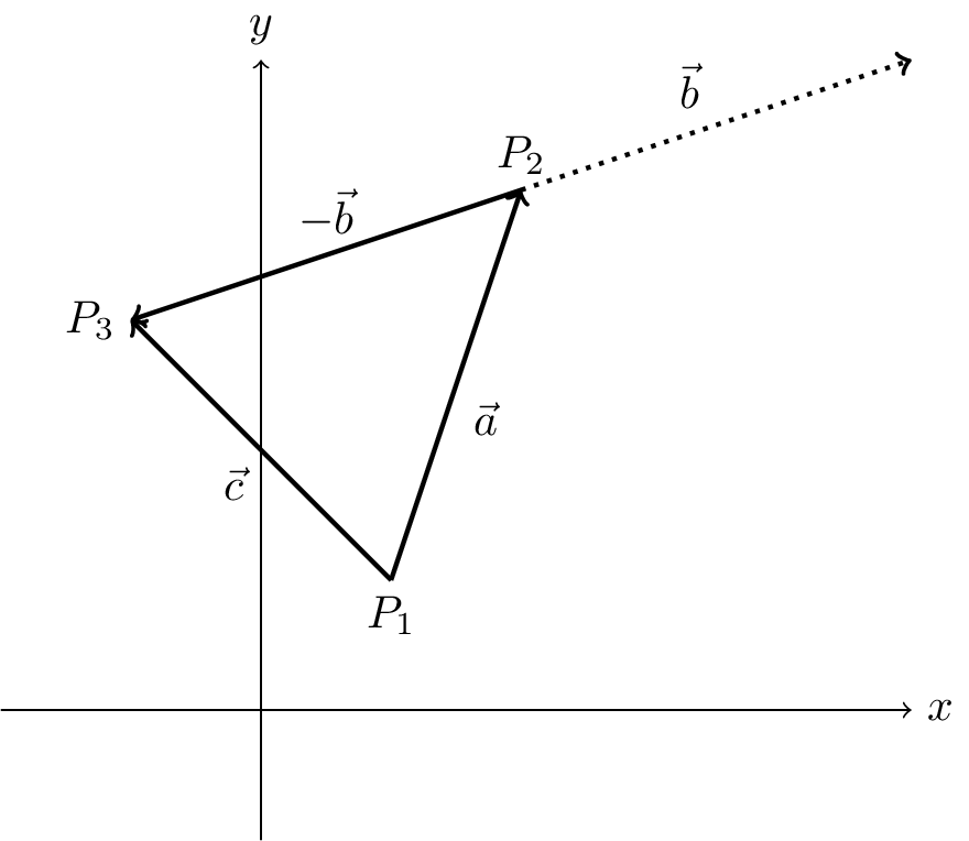
You can think of vectors as lines with a particular length and direction (see Figure 3.1). These could be displacement vectors representing the distance and direction between two points in space.

We will write vectors with an arrow above them, e.g., \(\vec{a}\), but you might also see vectors written in bold, \(\mathbf{a}\), or underlined, \(\underline{a}\). It doesn’t matter what notation you use as long as you remain consistent and are clear about which quantities are vectors, and which are regular numbers or scalars.
Vectors are quantities that have both a magnitude and a direction that can be added together like displacements (see Figure 3.1).
There are several important properties that vectors have that you should be familiar with.
3.1.2 Magnitude
The magnitude of a vector is its length. The magnitude of the vector \(\vec{a}\) is a scalar, \(a\), which is written as \[ a = \left| \vec{a} \right|. \]
3.1.3 Multiplication by a scaler
Multiplying a vector by a scalar produces another vector that is parallel to the original vector, but with a different magnitude. \[ \vec{b} = \lambda \vec{a} \] where \(\lambda\) is a scalar. The magnitude of this new vector is \[ b = \left| \vec{b} \right| = \left| \lambda \vec{a} \right| = \left| \lambda \right| \left| \vec{a} \right| = \left| \lambda \right| a. \] The direction of the new vector is the same as the original vector (i.e., parallel) if \(\lambda > 0\), and opposite (i.e., anti-parallel) if \(\lambda < 0\).
3.1.4 Unit vector
A vector that has length \(1\) is said to be a unit vector. We can convert a vector to a unit vector by dividing by its length (equivalent to multiplying by 1 / length). We denote a unit vector by writing a “hat” over the vector.
\[ \hat{a} = \frac{\vec{a}}{|\vec{a}|}, \] which has magnitude 1, \[ |\hat{a}| = 1. \]
3.1.5 Addition and subtraction of vectors
We have seen how to add vectors in Figure 2.1. The sum of two vectors is another vector. The sum of two vectors \(\vec{a}\) and \(\vec{b}\) is written as \[ \vec{c} = \vec{a} + \vec{b}. \]
Subtracting \(\vec{b}\) from \(\vec{a}\) can be achieved by adding \(-1 \times \vec{b} = -\vec{b}\) to \(\vec{a}\). This is illustrated in Figure 3.2. \[ \vec{c} = \vec{a} - \vec{b} = \vec{a} + (-\vec{b}). \]
3.1.6 Summary of vector properties
There are important algebraic rules that vectors obey. These are:
- Commutative law \[ \vec{a} + \vec{b} = \vec{b} + \vec{a}. \]
- Associative law \[ (\vec{a} + \vec{b}) + \vec{c} = \vec{a} + (\vec{b} + \vec{c}). \]
- Distributive law \[ \alpha (\vec{a} + \vec{b}) = \alpha \vec{a} + \alpha \vec{b} \] where \(\alpha\) is a scalar.
These might seem obvious for vectors, but you will encounter other objects later on that do not obey these rules. You can try to prove these, e.g., by sketching a diagram.
3.2 Components of a vector
So far we have considered vectors as directed line segments without specific reference to any coordinate system. Everything we have defined so far is independent of any coordinate system. This is one of the benefits of using vectors. However, we often want to calculate quantities in a specific frame of reference, with a particular coordinate system. To do this we can write the components of a vector in terms of a coordinate system.
As a concrete example we will look first at cartesian coordinates in two dimensions. We can get the \(x\)-component of a vector by projecting the vector onto the \(x\)-axis. Similarly, we can obtain the \(y\)-component by projecting the vector onto the \(y\)-axis. This is illustrated in Figure 3.3.
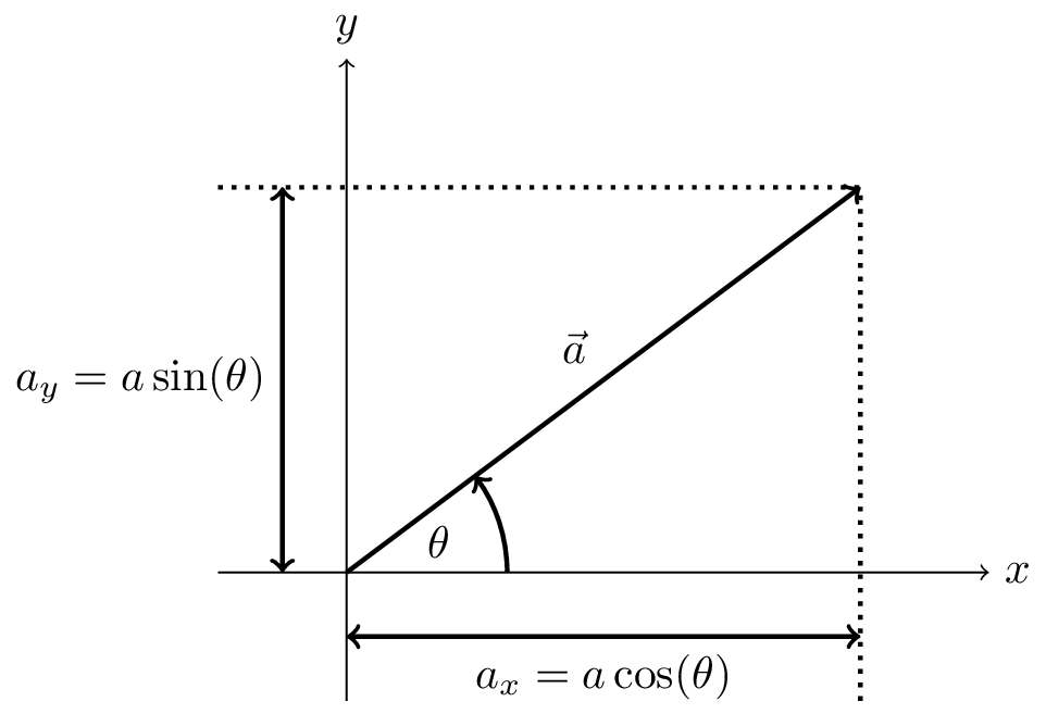
We can also see from the figure that the angle between the vector \(\vec{a}\) and the \(x\)-axis is given by \[ \tan(\theta) = \frac{a_y}{a_x} \] and the magnitude of \(\vec{a}\) is given by \[ \left| \vec{a} \right| = \sqrt{a_x^2 + a_y^2} \] using Pythagoras’ theorem.
3.2.1 Basis unit vectors
In cartesian coordinates in three dimensions we denote unit vectors in the \(x\), \(y\), and \(z\) directions as \(\hat{\imath}\), \(\hat{\jmath}\), and \(\hat{k}\), respectively. These are called basis vectors. Any vector can be written as a linear combination of scalars times these basis vectors. For example, the vector \(\vec{a}\) can be written as \[ \vec{a} = a_x \hat{\imath} + a_y \hat{\jmath} + a_z \hat{k}. \] where \(a_x\), \(a_y\), and \(a_z\) are the components of the vector \(\vec{a}\) in the \(x\), \(y\), and \(z\) directions, respectively. This is illustrated in Figure 3.4.
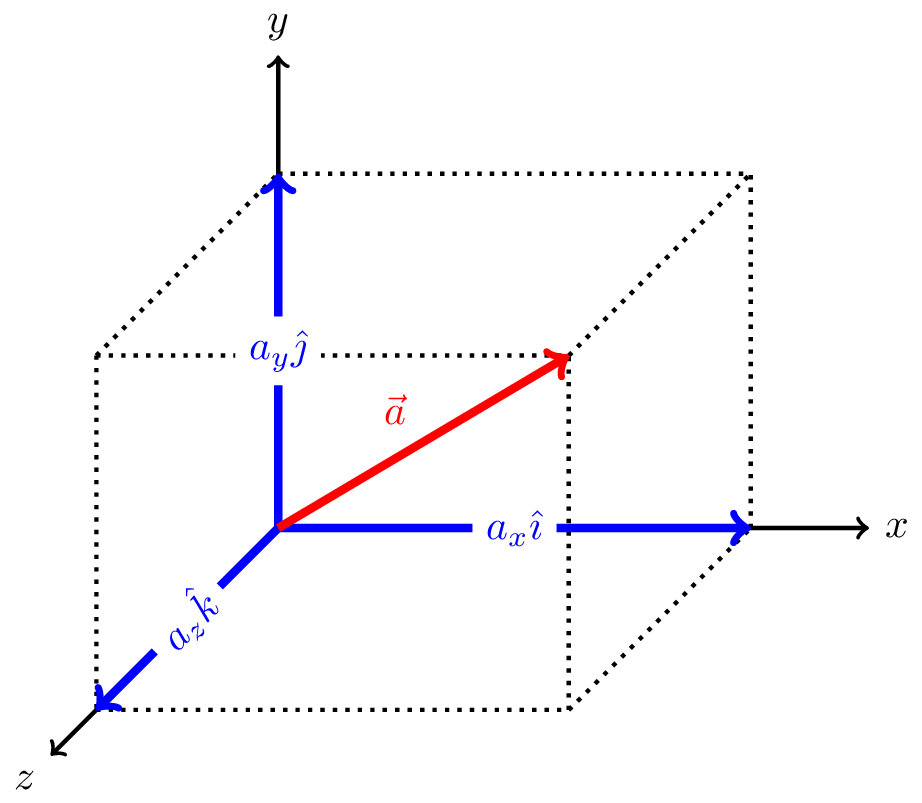
We can also write the vector \(\vec{a}\) as \[ \vec{a} = (a_x, a_y, a_z) \] where the components of the vector are written in parentheses. This is called the component form of the vector.
One way to determine these components is using direction cosines by looking at the component of the vector projected onto the coordinate axes. The components of \(\vec{a}\) are given by \[ a_x = |\vec{a}| \cos(\alpha) \] \[ a_y = |\vec{a}| \cos(\beta) \] \[ a_z = |\vec{a}| \cos(\gamma) \] where \(\alpha\), \(\beta\), and \(\gamma\) are the angles between \(\vec{a}\) and the \(x\), \(y\), and \(z\) axes, respectively.
3.3 Vector position, velocity, and acceleration
The position vector of a particle is its vector displacement from the origin. The position vector of a particle at position \((x, y, z)\) is given by \[ \vec{r} = x \hat{\imath} + y \hat{\jmath} + z \hat{k}. \]
A change in position for a particle moving from position vector \(\vec{r}_0\) at time \(t_0\) to \(\vec{r}_1\) at time \(t_1\) is given by \[ \Delta \vec{r} = \vec{r_1} - \vec{r_0}. \]
The average velocity vector is then \[ \vec{v}_\text{av} = \frac{\Delta \vec{r}}{\Delta t} \] where \(\Delta t = t_1 - t_0\). This closely follows our discussion of velocity in one dimension.
The instantaneous velocity is then given by \[ \vec{v} = \lim_{\Delta t \to 0} \frac{\Delta \vec{r}}{\Delta t} = \frac{d\vec{r}}{dt} = \dot{\vec{r}}. \]
3.4 Relative velocity
This is a generalisation fo the one dimensional case, where the scalars have been replaced by vectors.
\[ \vec{v}_\text{p} = \vec{v}_\text{t} + \vec{v}_\text{tp} \]
A pilot wants to land a plane on a runway heading due north. The speed of the plane relative to the air is \(70 \text{ m s}^{-1}\). There is a cross-wind of \(15 \text{ m s}^{-1}\) blowing from the west to the east. What direction should the pilot point the plane to land on the runway? How fast is the plane moving relative to the ground?

The wind will tend to blow the plane off course to the east. To compensate for this the pilot has to have some component of their motion into the wind. This is illustrated in Figure 3.5. We can see that the velocity of the plane relative to the ground, \(\vec{v}_\text{pg}\), is given by \[ \vec{v}_\text{pg} = \vec{v}_\text{pa} + \vec{v}_\text{ag}. \] The desired angle is then given by \[ \sin(\theta) = \frac{|\vec{v}_\text{ag}|}{|\vec{v}_\text{pa}|} = \frac{v_\text{ag}}{v_\text{pa}} = \frac{15}{70} = 0.214. \] \[ \theta = 12.1^\circ. \]
We can use Pythagoras’ theorem to calculate the speed of the plane relative to the ground, \[ v_\text{pg} = \sqrt{v_\text{pa}^2 - v_\text{ag}^2} = \sqrt{70^2 - 15^2} = 68.4 \text{ m s}^{-1}. \]
3.5 Summary
Position \[\vec{x}(t)\] Velocity \[\vec{v}(t) = \frac{d\vec{x}}{dt} = \dot{\vec{x}}\] Acceleration \[\vec{a}(t) = \frac{d\vec{v}}{dt} = \frac{d^2\vec{x}}{dt^2} = \ddot{\vec{x}}\] Note: we will use the convention that “speed” is a scalar and “velocity” as a vector.